TV Ratings From IMDB
Introduction
This is a follow up to a previous post about graphing X Files episodes ratings. In this post, I will generalize the method and clean up the code to subset the IMDB ratings data to almost any show in the IMDB ratings file. The ratings file can be found at IMDB Interfaces.
Data
Opening the ratings file in a text editor we can see it looks like this:
# New   Distribution  Votes  Rank  Title
# 0000013201    1294   7.5  "The X Files" (1993) {2Shy (#3.6)}
This has a mix of tab and space deliminated and will have to be cleaned up before the data frame is created.
Function
get.IMDB.data <- function(fP, showName) {
  imdb.text <- readLines(fP) # Read in data
  # tv show data is indicated by wrapping the episode name and season episode number in a {}
  imdb.dat <- imdb.text[grepl(showName, imdb.text, ignore.case=T) & grepl("}", imdb.text)]
  if (length(imdb.dat) == 0) {
      stop(paste(showName, "was not found, please check IMDB about possible name"))
    } else {
      imdb.dat <- gsub("\\)", "", gsub("\\(", "", imdb.dat))

      # Really need to clean up the values in the {}, so do that now
      imdb.dat <- gsub("\\{", "\\\"", imdb.dat) # replace the { with \"
      imdb.dat <- gsub("(.*)\\#(.*)", "\\1\\\" \\2", imdb.dat, perl=T) # replace the LAST # with \" to create quoted line eg foo bar becomes "foo bar" so when reading it in the "foo bar" is treated as one word
      imdb.dat <- gsub("\\}", "", imdb.dat) # Remove the } as not needed anymore
      imdb.dat <- gsub("(.*)\\.(.*)", "\\1 \\2", imdb.dat, perl=T) # replace the LAST . with " " to split season and episode #
      imdb.dat <- gsub("\\s+", " ", sub("^\\s+", "", imdb.dat)) # Remove leading and trailing whitespace

      # Create data frame
      imdb.df <- read.table(text=imdb.dat, sep=" ", header=F) # read the data into a data frame
      names(imdb.df) <- c("Distribution", "Votes", "Rate", "Title", "Year", "Epi.Name", "Season.Num", "Episode.Num") # add column names
      imdb.df <- imdb.df[grepl(showName, imdb.df$Title, ignore.case=T),] # Clean up so only shows with the name are included
      imdb.df <- imdb.df[order(imdb.df$Title, imdb.df$Year, imdb.df$Season.Num, imdb.df$Episode.Num),] # sort by titale -> year -> season -> epi num
      return(imdb.df)
    }
  }

fp <- "C:\\code\\web\\2015-05-18-XFiles-Season-Rating/ratings.list"
showName <- "The Wire"

show.data <- get.IMDB.data(fp, showName)
Unfortunately with this implementation, the show title must be a very close match. Cases are ignored but a show like Star Trek: The Next Generation will not be found if the ‘:’ is missing from Trek. Although there is an error catch, searching should be improved in a future version.
Checking the data
Show Titles
One of the first values to be checked is that it did not grab any extra shows:
kable(data.frame(table(as.character(show.data$Title))), align="c")| Var1 | Freq |
|---|---|
| Hot Off the Wire | 1 |
| The Wire | 60 |
| The Wire: The Chronicles | 3 |
From this, can easily extract our data:
show.data <- show.data[show.data$Title == "The Wire",]

kable(data.frame(table(as.character(show.data$Title))), align="c")| Var1 | Freq |
|---|---|
| The Wire | 60 |
Seasons
We should also check that all seasons are present. Now this is more tricky with regards to the given data set. Since we do not know how many seasons there are, we will assume that the greatest value, is the total number of seasons. This simplifies it, but again if last season is missing, we will not know using this data set and other sources would need to be used to verify (check IMDB or the shows Wikipedia entry).
The ‘%in%’ statement compares the values of the first vector to all the values in the second vector for matches. [1,2,3] %in% [2,5] would return [FALSE, TRUE, FALSE], using this we can check the seasons.
sum(!(1:max(show.data$Season.Num) %in% show.data$Season.Num))## [1] 0Since the sum of not found seasons is 0, we can assume we have all the seasons present in the data set.
Episodes
Again, we can use this same idea to check the episode numbering. As before, we will make the assumption that the total number of episodes in a season is the same as the maximum episode number for the respective season. To double check, we would need to use another source of data (IMDB, Wikipedia, etc.).
For this the plyr package will be used to make it much simpler.
library(plyr)

ep.check <- ddply(show.data, .(Season.Num), summarize, epi.miss=sum(!(1:max(Episode.Num) %in% Episode.Num)))

kable(ep.check, align="c")| Season.Num | epi.miss |
|---|---|
| 1 | 0 |
| 2 | 0 |
| 3 | 0 |
| 4 | 0 |
| 5 | 0 |
From this and the assumptions made, we can say we have all the seasons and episodes for the show.
Graphs
Lets generate the graphs like the X Files post, one thing to note is that to use the colour brewer, the colour variable should be a factor.
library(ggplot2)

# Generate line graph
ggplot(show.data, aes(x=1:nrow(show.data), y=Rate, colour=factor(Season.Num), group=Season.Num)) + geom_line(size=1) + geom_point(size=4, shape=21, fill="white") + xlab("") + scale_colour_brewer(palette="Paired") + ggtitle("Ratings of The Wire")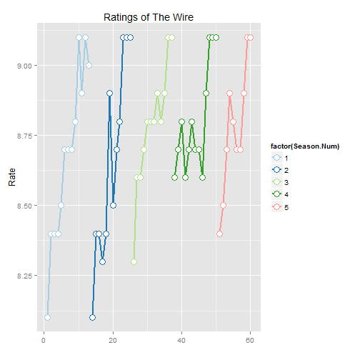
# Generate bar graph
ggplot(show.data, aes(x=Season.Num, y = Rate, colour=factor(Season.Num), group=Season.Num)) + geom_boxplot(fill=NA) + geom_point() + xlab("") + scale_colour_brewer(palette="Paired") + ggtitle("Ratings of The Wire by season")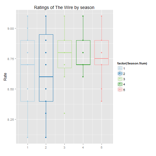
Conclusion
Hopefully, this is a much clearer version than the previous post and maybe learned something about R.
As a last bit, the session info:
sessionInfo()## R version 3.2.0 (2015-04-16)
## Platform: x86_64-w64-mingw32/x64 (64-bit)
## Running under: Windows 7 x64 (build 7601) Service Pack 1
##
## locale:
## [1] LC_COLLATE=English_United States.1252
## [2] LC_CTYPE=English_United States.1252
## [3] LC_MONETARY=English_United States.1252
## [4] LC_NUMERIC=C
## [5] LC_TIME=English_United States.1252
##
## attached base packages:
## [1] stats graphics grDevices utils datasets methods base
##
## other attached packages:
## [1] ggplot2_1.0.1 plyr_1.8.2 knitr_1.10
##
## loaded via a namespace (and not attached):
## [1] Rcpp_0.11.6 digest_0.6.8 MASS_7.3-40
## [4] grid_3.2.0 gtable_0.1.2 formatR_1.2
## [7] magrittr_1.5 evaluate_0.7 scales_0.2.4
## [10] highr_0.5 stringi_0.4-1 reshape2_1.4.1
## [13] labeling_0.3 proto_0.3-10 RColorBrewer_1.1-2
## [16] tools_3.2.0 stringr_1.0.0 munsell_0.4.2
## [19] colorspace_1.2-6