Replicating U Shaped Vehicle Crash Statistic
Introduction
With the aging population in North America, one of the most cited issues is about the U shaped trend of crash fatalities compared to age. One of the papers that highlights this was back in 1993 American Journal of Epidemiology by Leonard Evans where younger drivers had a higher crash risk that decreased with age and increasing again as people got older. Although this is not saying older drivers are more unsafe but other factors such as being more frail and impacts that a younger person would walk away from it would be fatal for an older person.
Data
FARS
The crash data was obtained from the Fatality Analysis Reporting System (FARS) using the persons database file. This has a variety of information including:
- INJ_SEV: Injury Severity
- AGE: Age of the person
- SEX: Male or Female
- PER_TYP: Role of the person in crash, e.g. driver, passenger, pedestrian, etc.
In order to read the data, the foreign package will be used and more precisely the function read.dbf to import the data.
library(foreign)

read.in <- function(fP) {
  df <- NA
  if (file.exists(fP)) {
    df <- read.dbf(file=fP, as.is=T)
  } else {
    stop(paste("File does not exist:", fP))
  }
  return(df)
}
Census
Population data was taken from CDC Bridge-Race Population Estimates. This provides yearly population data of from the United States based on Age and Gender.
The files are formatted as tab deliminated and have some extra information at the bottom of the file that needs to be removed.
## Census from http://wonder.cdc.gov/bridged-race-population.html
read.census <- function(fP) {
  if (file.exists(fP)) {
    census<- read.delim(fP, header=T, stringsAsFactors=F)
    # After '---' we dont need as seperates 'new' info, so lets get rid of it
    census <- census[1:(which(census == "---")[1]-1),]
    # Remove 'total'
    census <- census[which(census$Notes != "Total"),]
    return(census)
  } else {
    stop(paste("File does not exist:", fP))
  }
}
Crashes Per Million
To calculate crash per million by age, a histogram of all crashes is made first. After this the total population is divided into it and multiplied by a million.
The census data groups people 85 and over into one category, because of this anyone 85 and over will not be counted.
crash.per.mil <- function(per.df, sex, census, gen.code) {
  if (sex != 1 & sex != 2) {
    stop("Sex must be 1 or 2")
  }
  if (toupper(gen.code) != "M" & toupper(gen.code) != "F") {
    stop("Gender code must be 'M' or 'F'")
  }
  # Create histogram of data, num bins + 1 (85+1)
  his <- hist(per.df$AGE[per.df$PER_TYP == 1 & (per.df$SEX == sex) & per.df$INJ_SEV == 4 & per.df$AGE < 200], breaks=seq(0,84,l=86), plot=F)
  # Get population of gender
  cen.age <- census$Population[census$Gender.Code == toupper(gen.code)]

  # Only first 85 years are unique, after 85 it gets lumped into one
  c.p.m <- his$count / cen.age * 1000000
  return(c.p.m)
}
Using the functions above, the data for crashes per million can be calculated.
fars.base <- "C:\\code\\web\\2015-06-24-U-Shaped-Crash\\fars\\dbf"
cens.base <- "C:\\code\\web\\2015-06-24-U-Shaped-Crash\\fars\\Census"

get.crash.per.mil <- function(fP.fars, fP.census) {
  fars <- read.in(fP.fars)
  census <- read.census(fP.census)

  # Remove 85 or over
  fars <- fars[fars$AGE < 85,]
  census$Age.Code <- suppressWarnings(as.numeric(census$Age.Code))
  census <- census[!is.na(census$Age.Code),]

  c.p.m.M <- crash.per.mil(fars, 1, census, "M") # Male
  c.p.m.F <- crash.per.mil(fars, 2, census, "F") # Female

  df <- data.frame(age=rep(0:84,2), sex=c(rep("M", length(c.p.m.M)), rep("F", length(c.p.m.F))), crash.per.mil=c(c.p.m.M, c.p.m.F))
}

## 1990
fP.fars.1990 <- paste0(fars.base, "/", "person1990.dbf")
fP.cens.1990 <- paste0(cens.base, "/", "Bridged-Race Population Estimates 1990.txt")
cpm.1990 <- get.crash.per.mil(fP.fars.1990, fP.cens.1990)

## 2000
fP.fars.2000 <- paste0(fars.base, "/", "person2000.dbf")
fP.cens.2000 <- paste0(cens.base, "/", "Bridged-Race Population Estimates 2000.txt")
cpm.2000 <- get.crash.per.mil(fP.fars.2000, fP.cens.2000)

## 2005
fP.fars.2005 <- paste0(fars.base, "/", "person2005.dbf")
fP.cens.2005 <- paste0(cens.base, "/", "Bridged-Race Population Estimates 2005.txt")
cpm.2005 <- get.crash.per.mil(fP.fars.2005, fP.cens.2005)

## 2010
fP.fars.2010 <- paste0(fars.base, "/", "person2010.dbf")
fP.cens.2010 <- paste0(cens.base, "/", "Bridged-Race Population Estimates 2010.txt")
cpm.2010 <- get.crash.per.mil(fP.fars.2010, fP.cens.2010)

## 2013
fP.fars.2013 <- paste0(fars.base, "/", "person2013.dbf")
fP.cens.2013 <- paste0(cens.base, "/", "Bridged-Race Population Estimates 2013.txt")
cpm.2013 <- get.crash.per.mil(fP.fars.2013, fP.cens.2013)
Graphing
To graph the data the ggplot2 package will be used with age on x-axis and crashes per million on y-axis.
graph.crash <- function(df, year) {
  library(ggplot2)
  return(ggplot(df, aes(x=age, y=crash.per.mil, col=sex)) + geom_point() + xlab("Age") + ylab("Crashes per Million") + ggtitle(paste("Age vs Crashes per Million People, Year - ", year)) + scale_x_continuous(breaks=seq(0,85,5)))
}

## make graphs
p.1990 <- graph.crash(cpm.1990, 1990)
p.1990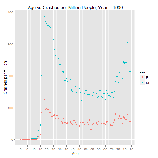
p.2000 <- graph.crash(cpm.2000, 2000)
p.2000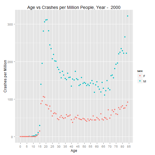
p.2005 <- graph.crash(cpm.2005, 2005)
p.2005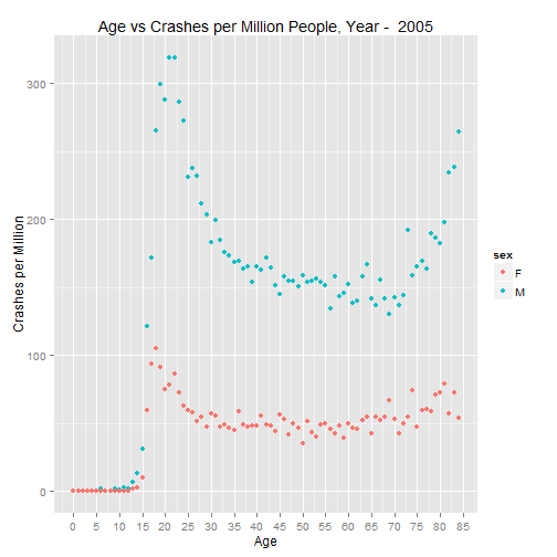
p.2010 <- graph.crash(cpm.2010, 2010)
p.2010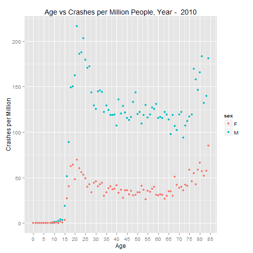
p.2013 <- graph.crash(cpm.2013, 2013)
p.2013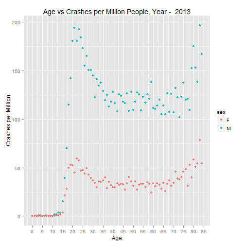
Conclusion
As was the case in the paper, the U shaped trend continues in recent years.