Visualizing Traffic Signals with PostGIS, OSM, and R
This was my first introduction to PostGIS with Open Street Map data. Although the use of the information between this post and my original need, I always liked the picture you could make by mapping a cities traffic signals.
Data
In order to get city information, Open Street Map (OSM) data will be used for the City of Winnipeg and can be downloaded from Mapzen Metro Extracts.
If you need to set up PostGIS and osm2pgsql using Windows I wrote a very quick guide here that will point you to specific a osm2pgsql build and library that has worked for me on 64 bit Windows 7 and 10.
Open Street Map Keys and Values
Open Street Map uses a Key and Value to store information such as traffic signals. From the OSM wiki, the traffic signals for vehicular traffic can be found. Other important information such as, how it is tagged, pedestrian crossing, and more can be found on the Wiki.
From the OSM Wiki, traffic signals only used by vehicular traffic can be obtained by querying for the Key as ‘highway’ and the Value as ‘traffic_signals’.
Open Street Map Projection
The projection system used by OSM is Spherical Mercator (EPSG: 3857) and since we want to plot with latitude and longitude, it must be changed to EPSG: 4326. Luckily PostGIS function ST_Transform will do this for us.
Create Visualization
In order to communicate with the PostGIS database, the RPostgreSQL package will be used. Plotting will be done through the ggplot2 package.
library(RPostgreSQL) # Aquiring Data from DB

library(ggplot2) # Used for Plotting
RPostgreSQL Connection
The following will form the connection between R and the PostGIS database, ‘gis’. This will allow SQL statements to be sent and results to be fetched from the PostGIS database.
m <- dbDriver("PostgreSQL")
con <- dbConnect(m, dbname="gis")
Create Query
To get the latitude and longitude of each traffic signal, the planet_osm_point table is used. The way The criteria to be queried is where the key is highway and tag of ‘traffic_signals’.
The following are PostGIS functions:
- ST_X/Y acquires the X or Y coordinate of a point.
- ST_Transform will transform a geometry from one coordinate to another.
Combining this information into the SQL command below, dbGetQuery will query the connection and return the answer to the query as a data frame.
q <- "SELECT
      highway as Tag,
      ST_Y(ST_Transform(way,4326)) AS lat,
      ST_X(ST_Transform(way,4326)) AS lon
      FROM planet_osm_point
      WHERE highway = 'traffic_signals'"
ts <- dbGetQuery(con, q) # Data frame of all traffic signals

# Display first few rows of traffic signal df

kable(head(ts), align='c')| tag | lat | lon |
|---|---|---|
| traffic_signals | 49.87586 | -97.40278 |
| traffic_signals | 49.87597 | -97.40276 |
| traffic_signals | 49.87533 | -97.38807 |
| traffic_signals | 49.87551 | -97.38806 |
| traffic_signals | 49.87640 | -97.36107 |
| traffic_signals | 49.87625 | -97.36102 |
Plotting
To make the visualization, the graph will be completely black with only the traffic signal locations showing as white dots.
To black out the plot, the theme function of ggplot2 is used. The panel background and plot background are filled with a black rectangle. The grids are blanked out and lines removed with element_blank.
theme(panel.background = element_rect(fill = 'black', colour = 'black'), plot.background = element_rect(fill = 'black', colour = 'black'),
        panel.grid.major = element_blank(), panel.grid.minor = element_blank(), text = element_blank(), line = element_blank())
The last bit is to use coord_flip() to rotate the image to compass directions with north being up.
Combining the functions as below will produce the desired image:
ggplot(ts, aes(x=lat, y=lon)) + geom_point(col='white', size=0.5) +
  theme(panel.background = element_rect(fill = 'black', colour = 'black'), plot.background = element_rect(fill = 'black', colour = 'black'),
        panel.grid.major = element_blank(), panel.grid.minor = element_blank(), text = element_blank(), line = element_blank()) + coord_flip()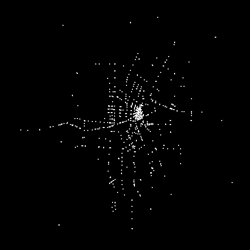
Traffic Signals in Canada
The last bit will be to extend the above to graph all of Canada that has traffic signal information. The data was gathered from Geofabrik and loaded into a seperate database.
The same query can be made to obtain all traffic signal locations.
con2 <- dbConnect(m, dbname="gisdb")
q <- "SELECT
      highway as Tag,
      ST_Y(ST_Transform(way,4326)) AS lat,
      ST_X(ST_Transform(way,4326)) AS lon
      FROM planet_osm_point
      WHERE highway = 'traffic_signals'"
can_ts <- dbGetQuery(con2, q) # Data frame of all traffic signals
An extra step will be taken to get all the lines making up Canada’s boundary. To do this, ST_DumpPoints will dump out all points transformed to lat lon. The other part, is to get province boundaries. According to OSM Wiki here admin level of 4 must be used. The points will be ordered to form a lines.
q2 <- "SELECT (dp).path[1], (dp).path AS index, ST_Y((dp).geom) AS lat, ST_X((dp).geom) AS lon
FROM (SELECT ST_DumpPoints(ST_Transform(way, 4326)) AS dp
FROM planet_osm_line where boundary='administrative' and admin_level = '4') AS foo
ORDER BY index;"
cb <- dbGetQuery(con2, q2)
Now combining this all, a map of Canada can be produced with all traffic signals.
ggplot(can_ts, aes(x=lat, y=lon)) + geom_point(col='white', size=0.5) + geom_point(data=cb, aes(x=lat, y=lon), col='red', size=0.5, alpha=0.01) +
  theme(panel.background = element_rect(fill = 'black', colour = 'black'), plot.background = element_rect(fill = 'black', colour = 'black'),
        panel.grid.major = element_blank(), panel.grid.minor = element_blank(), text = element_blank(), line = element_blank()) + coord_flip()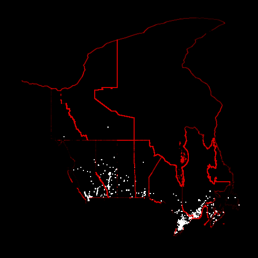
The province boarders were plotted using the points instead of lines.
Conclusion
PostGIS, OSM, and R continue to be powerful tools for doing GIS information and hopefully this proves useful.