Drawing Polygons with PostGIS, Open Street Maps, and R
Introduction
Working with maps, its nice to be able to display the map with additional information. In a previous post, it showed how to get points, but unforunately the method does not properly export data drawing the regions. This post will correct that and using R the regions will be plotted properly.
PostGIS
In order to get ordered points that form the region, a sub function must be used to extract the points from planet-osm-polygon while perserving the order. This is achieved through the ST_DumpPoints and ST_Collect functions.
ST_DumpPoints, will return the points from the geometry as well as a path indicating the index of the point on the polygon. The path supplies an index where first value is the shape it belongs to (region) and the second value corresponds to which in order point it is, e.g. {1,1}, {1,2}, {2,1},{2,2},{2,3}.
ST_Collect gathers all values from the geometry for a particular set and returns it. This will distinguish different regions in ST_DumpPoints.
Combining both ST_DumpPoints and ST_Collect to gather the information from the province level boundaries of the Canada information give:
SELECT ST_DumpPoints(ST_Collect(way)) AS dp
 FROM  planet_osm_polygon where boundary='administrative' and admin_level = '4') AS foo
Using the path will return the region and order, ST_X/Y will transform the points to lat/lon. The region can be extracted using path[1] and the region and order can be passed back using path on the dumped points (dp).
SELECT (dp).path[1] AS region, (dp).path AS index, ST_X((dp).geom) AS lon, ST_Y((dp).geom) AS lat
FROM (SELECT ST_DumpPoints(ST_Collect(way)) As dp
 FROM  planet_osm_polygon where boundary='administrative' and admin_level = '4') As foo
ORDER BY index;
PostGIS and R
In order to send and receive commands to PostGIS, the package RPostgreSQL will be used. Connecting to the database, then can be done using dbDriver and dbConnect .
Using this, the query can be generated and passed to the PostGIS database using the dbGetQuery command and the answer to the query will be as a data frame.
library(RPostgreSQL)

# Connect to database
m <- dbDriver("PostgreSQL")
con <- dbConnect(m, dbname="gisdb")

# Create query
q <- "SELECT (dp).path[1] AS region, (dp).path AS index, ST_X((dp).geom) AS lon, ST_Y((dp).geom) AS lat
FROM (SELECT ST_DumpPoints(ST_Collect(way)) AS dp
 FROM  planet_osm_polygon where boundary='administrative' and admin_level = '4') AS foo
ORDER BY index;"

# Send query to PostGIS and receive results
regions <- dbGetQuery(con, q)

# Look at information
kable(rbind(head(regions), tail(regions)), align='c')| region | index | lon | lat | |
|---|---|---|---|---|
| 1 | 1 | {1,1,1} | -79.77413 | 54.63557 |
| 2 | 1 | {1,1,2} | -79.77290 | 54.63797 |
| 3 | 1 | {1,1,3} | -79.77065 | 54.64236 |
| 4 | 1 | {1,1,4} | -79.76943 | 54.64471 |
| 5 | 1 | {1,1,5} | -79.76650 | 54.64597 |
| 6 | 1 | {1,1,6} | -79.76015 | 54.64868 |
| 256415 | 19 | {19,1,19028} | -95.15366 | 52.54417 |
| 256416 | 19 | {19,1,19029} | -95.15366 | 52.56387 |
| 256417 | 19 | {19,1,19030} | -95.15366 | 52.58688 |
| 256418 | 19 | {19,1,19031} | -95.15366 | 52.60279 |
| 256419 | 19 | {19,1,19032} | -95.15366 | 52.62336 |
| 256420 | 19 | {19,1,19033} | -95.15374 | 52.62364 |
Now that the regions are given to us, all that is left is to plot each region. To do this, the plot will be created based on the ranges of the lat/lon of the file and then plot each region by iterating through them.
plot(x="", xlim=range(regions$lon), ylim=range(regions$lat), xlab="Longitude", ylab="Latitude", main="OSM Canada Administrative Boundary 4")
uRegions <- unique(regions$region)
# Probably can be done without the loop
for (k in 1:length(uRegions)) {
  theRegion <- uRegions[k]
  lines(regions$lon[regions$region == theRegion], regions$lat[regions$region == theRegion])
}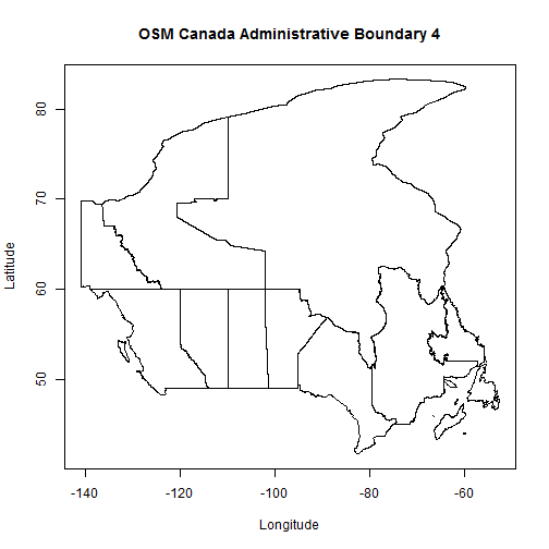
Note: This is missing New Brunswick, and alternative query that will include New Brunswick using the planet_osm_line can be done as below:
SELECT (dp).path[1] AS region, (dp).path AS index, ST_Y((dp).geom) AS lat, ST_X((dp).geom) AS lon
FROM (SELECT ST_DumpPoints(ST_Collect(way)) AS dp
FROM planet_osm_line where boundary='administrative' and admin_level = '4') AS foo
ORDER BY index;
The only difference is that planet_osm_line is used compared with planet_osm_polygon, though some gaps may appear.