Billboard Hot 100 Historical Lyrics, Quick Look
Introduction
Sometime ago, I wanted to analyse the lyrics in the Billboard Hot 100 over multiple years but never really knew what I wanted to actually look at. Recently, I scraped lyric data from a few websites to compile a complete set of lyrics from 1951 to 2015 and will look at average unique words through the years, although early years had ~30 songs. This has also let me play around with a few text mining packages, tm and SnowballC, although the later didn’t really use for this.
Most of the work for this was scraping and formatting the lyrics into a consistent format but that will not be shown here. The Billboard Hot 100 artist and song name was gathered from Wikipedia for years 1951-2015 and lyrics from various sources.
A Look at the Data
First, import the libraries to be used:
library(tm)
library(knitr)
library(ggplot2)
library(wordcloud)
Setup
What we want to do is read each lyric and store it as a PlainTextDocument object to be used with tm. From that, the data can be cleaned and extracted for analysis.
# Data was part of a data frame before hand and was read in already
doc.vec <- VectorSource(top100$lyrics)
doc.corp <- Corpus(doc.vec)
First step is to set everything to lowercase:
doc.corp <- tm_map(doc.corp, content_transformer(tolower))One issue that may be encountered is common words such as “you”, “a”, “the”, and such might want to be removed. A list of common words in english can be found using stopwords(“en”). Though, this can be done like before:
#doc.corp <- tm_map(doc.corp, removeWords, stopwords("en"))Now, remove all the remove punctuations.
doc.corp <- tm_map(doc.corp, removePunctuation)Removing all common words may not be what we want since words like “you” and “me” can define the song. By removing punctuation, the removed words should also have punctuation removed as well. With this, some common words can be removed:
doc.corp <- tm_map(doc.corp, removeWords, c("to","too", "i", "its","ill", "im", "a", "an", "and", "at", "are","on", "be", "the", "that", "for"))Next part is to strip extra white space:
doc.corp <- tm_map(doc.corp, stripWhitespace)Now to create a Document Term Matrix which will be used for analysis.
dtm <- DocumentTermMatrix(doc.corp)This now provides us with a basis to examin the lyrics with.
It is VERY IMPORTANT to note that the minimum word length is set to 3 by default. To change it, the call would be DocumentTermMatrix(doc.corp, control=list(wordLengths=c(1,Inf)) ), where 1 can be replaced with any minimum length.
There is much more that could of been done, such as stemming using the SnowballC package to remove affixes like “ing”, “ies”, and such from words to get at a root word. As well, could try to remove all common words provided by the stopwords(“en”) function.
Total Words
Using the Document Term Matrix, each row of the matrix:
top100$totWords <- rowSums(as.matrix(dtm))

ggplot(top100, aes(x=year, y=totWords)) + geom_boxplot() + theme(axis.text.x=element_text(angle=90, hjust=1, vjust=0.5))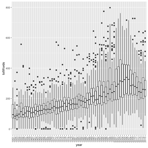
The issue with this, is that certain songs may repeat the chorus multiple times but adding no more unique words.
Total Unique Words
dtm.m <- as.matrix(dtm)
dtm.m[dtm.m > 0] <- 1
top100$totUWords <- rowSums(dtm.m)

ggplot(top100, aes(x=year, y=totUWords)) + geom_boxplot() + theme(axis.text.x=element_text(angle=90, hjust=1, vjust=0.5))
Lets take a look at which songs had over 300 unique words:
kable(top100[top100$totUWords > 300, c(1,2,5,10,11)], align='c', row.names=F)| Artist | Title | year | Total Words | Total Unique Words |
|---|---|---|---|---|
| Bad Meets Evil | Lighters | 2011 | 563 | 317 |
| Bill Hayes | The Ballad of Davy Crockett | 1955 | 557 | 314 |
| Dem Franchize Boyz | I Think They Like Me | 2006 | 716 | 325 |
| Drake | Forever | 2009 | 727 | 355 |
| Drake | Forever | 2010 | 727 | 355 |
| Eminem | Sing for the Moment | 2003 | 588 | 316 |
| Eminem | The Real Slim Shady | 2000 | 697 | 308 |
| Ludacris | Pimpin All Over the World | 2005 | 651 | 316 |
| Luniz | I Got 5 on It | 1995 | 476 | 306 |
| Master P | Make Em Say Uhh | 1998 | 656 | 324 |
| Missy Elliott | Gossip Folks | 2003 | 516 | 321 |
| Mo Thugs | Ghetto Cowboy | 1999 | 542 | 312 |
| Puff Daddy | Been Around the World | 1998 | 798 | 377 |
| Puff Daddy | Victory | 1998 | 613 | 365 |
| The Game | How We Do | 2005 | 495 | 313 |
| The Notorious BIG | One More Chance | 1995 | 553 | 304 |
It seems that rap music takes up the spots.
Top 25 Most Frequent Words
To take a look at the top 25 most frequented words:
kable(as.data.frame(tail(sort(colSums(as.matrix(dtm))), n=25)), align='c', col.names=c("Frequency"))| Word | Frequency |
|---|---|
| out | 6290 |
| she | 6491 |
| one | 6521 |
| down | 6883 |
| want | 7094 |
| youre | 7837 |
| yeah | 8323 |
| this | 8567 |
| now | 8635 |
| what | 9273 |
| get | 9332 |
| can | 9337 |
| got | 9435 |
| when | 9788 |
| but | 10362 |
| with | 10601 |
| just | 11150 |
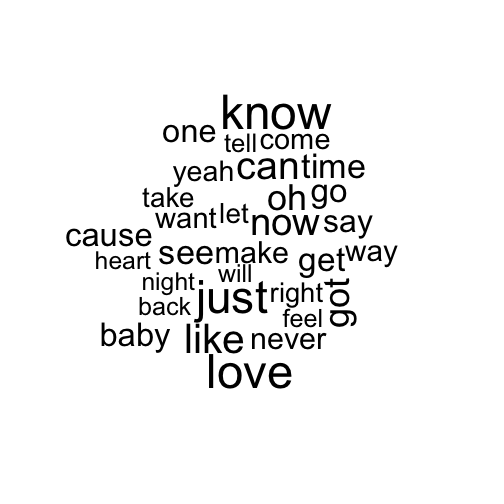
| baby | 11856 |
| like | 12258 |
| know | 13019 |
| all | 13946 |
| dont | 14010 |
| your | 17967 |
| love | 19155 |
| you | 77734 |
Since some frequent terms like you, your, youre, when, with, and other common terms are high up on the list, they should be removed at a later point and could be re-analysed. As well, minimum word length should be set to 1, then can do comparisons like ‘he’ vs ‘she’. At a later point I may look at this.
Update (2016-03-08) - Using stopwords(“en”) and Word Length 1 to Infinity
I wanted to give an update using stopwords(“en”) in full on this data set and word lengths from 1 to inifinity. Since the process is the same as above, I have not given much of
doc.vec <- VectorSource(top100$lyrics)
doc.corp <- Corpus(doc.vec)
# transform to lower then remove using stopwords
doc.corp <- tm_map(doc.corp, content_transformer(tolower))
# Remove all stop words
doc.corp <- tm_map(doc.corp, removeWords, stopwords("en"))
# Remove punctuation
doc.corp <- tm_map(doc.corp, removePunctuation)
# Remove extra white space
doc.corp <- tm_map(doc.corp, stripWhitespace)

# turn into document matrix
dtm.update <- DocumentTermMatrix(doc.corp, control=list(wordLengths=c(1,Inf)))

# Create with total words
dtm.update <- as.matrix(dtm.update)
top100$totWords.update <- rowSums(dtm.update)

ggplot(top100, aes(x=year, y=totWords.update)) + geom_boxplot() + theme(axis.text.x=element_text(angle=90, hjust=1, vjust=0.5))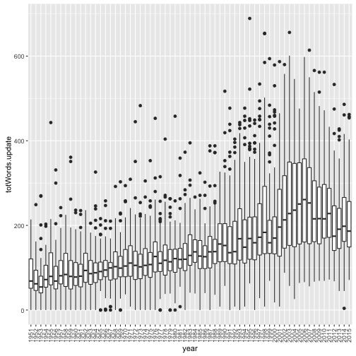
# Top 25 words
kable(as.data.frame(tail(sort(colSums(as.matrix(dtm.update))), n=25)), align='c', col.names=c("Frequency"))| Word | Frequency |
|---|---|
| gonna | 5358 |
| way | 5445 |
| never | 5670 |
| let | 5859 |
| girl | 5901 |
| say | 5916 |
| cause | 6012 |
| see | 6087 |
| make | 6155 |
| time | 6186 |
| come | 6189 |
| one | 6545 |
| want | 7115 |
| go | 7730 |
| yeah | 8332 |
| now | 8636 |
| can | 9337 |
| get | 9341 |
| got | 9439 |
| just | 11165 |
| baby | 11863 |
| like | 12263 |
| oh | 12996 |
| know | 13030 |
| love | 19163 |
# Create word cloud
wordcloud(names(dtm.update[1,]), colSums(as.matrix(dtm.update)), min.freq=4000)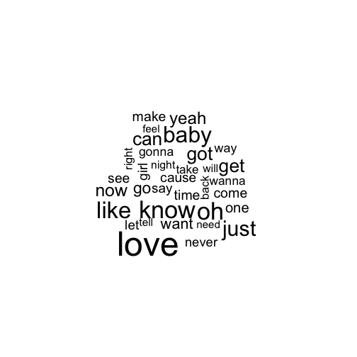
# Create total unique words
dtm.U <- as.matrix(dtm.update)
dtm.U[dtm.U > 0] <- 1
top100$totUWords.update <- rowSums(dtm.U)

ggplot(top100, aes(x=year, y=totUWords.update)) + geom_boxplot() + theme(axis.text.x=element_text(angle=90, hjust=1, vjust=0.5))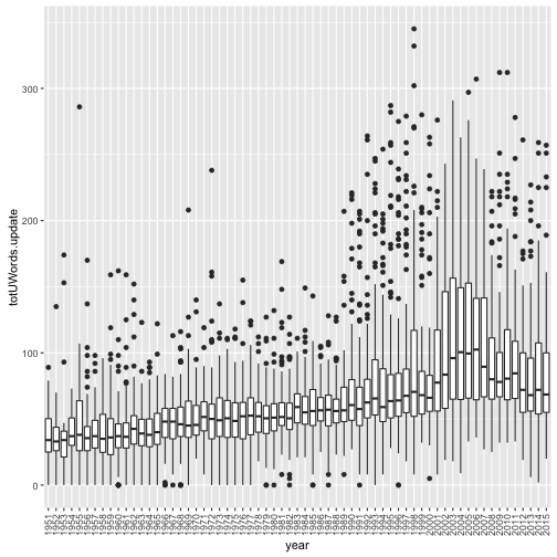
# Top 25 words
kable(as.data.frame(tail(sort(colSums(as.matrix(dtm.U))), n=25)), align='c', col.names=c("Frequency"))| Word | Frequency |
|---|---|
| right | 1784 |
| take | 1814 |
| let | 1824 |
| yeah | 1881 |
| come | 1908 |
| want | 1932 |
| way | 1977 |
| never | 2038 |
| make | 2043 |
| say | 2160 |
| one | 2208 |
| baby | 2229 |
| cause | 2233 |
| go | 2270 |
| get | 2280 |
| time | 2348 |
| see | 2362 |
| oh | 2503 |
| got | 2514 |
| now | 2708 |
| can | 2769 |
| like | 2910 |
| just | 3335 |
| love | 3449 |
| know | 3498 |
# Create word cloud
wordcloud(names(dtm.U[1,]), colSums(as.matrix(dtm.U)), min.freq=1500)